10 Ordinary Differential Equations
This chapter describes the functions for solving ordinary differential equation (ODE) initial value problems provided by the Science Collection. The functions include a variety of low-level methods, such as Runge-Kutta and Bulirsch-Stoer routines, and higher level components for adaptive step-size control. The components can be combined by the user to achieve the desired solution with full access to any intermediate steps, as needed.
The functions described in this chapter are defined in the "ode-initval.rkt" file in the Science Collection and are made available using the form:
10.1 Defining the ODE System
The routines solve the general n-dimensional first-order system:
dyi(t)/dt = fi(t, y1(t), ..., yn(t))
for i = 1, ..., n. The stepping functions rely on the vector of derivatives fi and the Jacobian matrix Jij = dfi(t, y(t))/dyj. A system of equations is defined using the ode-system structure.
Defines a general ODE system with arbitrary parameters.
function—a function (lambda (t y dydt params) ...). This function should store the elements of fi(t, y, params) in the vector dydt, for arguments t and y and parameters params.
jacobian—a function (lambda (t y dfdy dfdt params) ...). This function should store the elements of dfi(t, y, params)/dt in the vector dfdt and the Jacobian matrix Jij in the vector dfdy as a row-major matrix Jij = dfdy(i * dimension + j), where dimension is the dimension of the system. Some of the simpler solver algorithms do not make use of the Jacobian matrix, so it is not always strictly necessary to provide it. The jacobian field of the structure can be #f for those algorithms. However, it is useful to provide the Jacobian to allow the solver algorithms to be interchanged. The best algorithms make use of the Jacobian.
dimension—the dimension of the system of equations.
params—a list if the arbitrary parameters of the system.
Evaluates the system function for ode-system. This function should store the elements of fi(t, y, params) in the vector dydt, for arguments t and y and parameters params.
Evaluates the Jacobian function for ode-system. This function should store the elements of dfi(t, y, params)/dt in the vector dfdt and the Jacobian matrix Jij in the vector dfdy as a row-major matrix Jij = dfdy(i * dimension + j), where dimension is the dimension of the system.
10.1.1 Stepping Functions
The lowest level components are the stepping functions that advance a solution from time t to t + h for a fixed step size h and estimate the resulting local error.
Returns true, #t, if x is an ODE step type and false, #f, otherwise. ODE step types are defined by the different ODE solvers.
Returns true, #t, if x is an ODE step and false, #f, otherwise.
Returns a newly created instance of a stepping function of type step-type for a system of dim dimensions.
Resets the stepping function step. It should be used whenever the next use of step will not be a continuation of a previous step.
Returns the name of the stepping function step as a string.
Returns the order of the stepping function step on theprevious step. This order can vary of the stepping function itself is adaptive.
Applies the stepping function step to the system of equations defined by dydt using the step size h to advance the system from time t and state y to time t + h. The new state of the system is stored in y on output with an estimate of the absolute error in each component stored in y-err. If the argument dydt-in is not #f, it should be a vector containing the derivatives for the system at time t on input. This is optional as the derivatives will be computed internally if they are not provided, but allows the reuse of existing derivative information. On output the new derivatives of the system at time t + h will be stored in the vector dydt-out, if it is not #f.
The following stepping algorithms are available.
Embedded Runge-Kutta (2, 3) method.
4th order (classical) Runge-Kutta.
Embedded (classical) Runge-Kutta-Fehberg (4, 5) method. This method is a good general-purpose integrator.
10.2 Adaptive Step-Size Control
The control function examines the proposed changes to the solution and its error estimate produced by a stepping function and attempts to determine the optimal step size for a user-specified level of error.
Creates a new standard control object. The standard control object is a four parameter heuristic based on absolute and relative errors eps-abs and eps-rel and scaling factors a-y and a-dydt for the system state y{t} and derivatives y′(t), respectively.
The step size adjustment procedure for this method begins by computing the desired error level Di, for each component
Di = epsabs + epsrel × (ay|yi| + adydth|y′i|)
and comparing it with the observed error Ei = |yerri|. If the observed error E exceeds the desired error level D by more than 10% for any component, then the method reduces the step size by an appropriate factor
hnew = hold × S × (E/D)-1/q
where q is the consistency order of the method (e.g., q = 4 for 4(5) embedded RK), and S is a safety factor of 0.9. The ratio E/D is taken to be the maximim of the ratios Ei/Di.
If the observed error E is less than 50% of the desired level D for the maximum ratio Ei/Di, then the algorithm takes the opportunity to increase the step size to bring the error in line with the desired level
hnew = hold × S × (E/D)-1/(q+1).
This emcompasses all the standard scaling methods. To avoid uncontrolled changes in the step size, the overall scaling factor is limited to the range ⅕ to 5.
Creates a new control object that will keep the local error within an absolute error of eps-abs and relative error eps-rel with respect to the solution yi(t). This is equivalent to the standard control object with a-y = 1 and a-dydt = 0.
Creates a new control object that will keep the local error within an absolute error of eps-abs and relative error eps-rel with respect to the derivatives of the solution y′i(t). This is equivalent to the standard control object with a-y = 0 and a-dydt = 1.
Returns a new instance of a control function of type control-type. This function is only needed for defining new types of control functions. For most purposes, the standard control functions describes above should be sufficient.
Initializes the control function control with the parameters eps-abs (absolute error), eps-rel (relative error), a-y (scaling factor for y), and a-dydt (scaling factor for derivatives.)
Adjusts the step size h using the control function control and the current values of y, y-err, and dydt. The stepping function step is also needed to determine the order of the method. If the error in the y values y-err is found to be too large, then the step size h is reduced and the function returns -1. If the error is sufficiently small, then h may be increased and 1 is returned. The function returns 0 if the step size is unchanged. The goal of the function is to estimate the largest step size that satisfies the user-specified accuracy requirements for the current point.
Returns the name of the control function control. For example,
would print something like
control method is 'standard' |
10.3 Evolution
The highest-level of the system is the evolution function that combines the results of a stepping function and control function to reliably advance the solution forward over an interval (t0, t1). If the control function signals that the step size should be decreased, the evolution function backs out of the current step and tries the proposed smaller step size. This process is continued until an acceptable step size is found.
Returns true, #t, if x an ODE evolver.
Returns a new instance of an evolution function for a system of dim dimensions.
Returns the number of steps evolve has iterated.
Returns the number of steps for evolve that have failed — i.e., required adjustment to the time step.
Evolves the system from time t and position y using the stepping function step. The new time and position are stored in t and y on output. The initial step size is taken as h, but this may be modified using the control function control to achieve the appropriate bound, if necessary. The routine may make several calls to step in order to determine the optimum step size. If the step size has been changed, the value of h will be modified on output. The maximum time t1 is guaranteed not to be exceeded by the time step. On the final time step, the value of t will be set to t1 exactly.
Resets the evolution function evolve. It should be used whenever the next use of evolve will not me a continuation of a previous step.
10.4 ODE Examples
Example: The following programs solve the second-order nonlinear Van der Pol oscillator equation
x”(t) + μx′(t)(x(t)2 - 1) + x(t) = 0.
This can be converted into a first order system suitable for use with the routines described in this chapter by introducing a separate variable for the velocity, y = x′(t)
x′ = y
y′ = -r + μy(1 - x2).
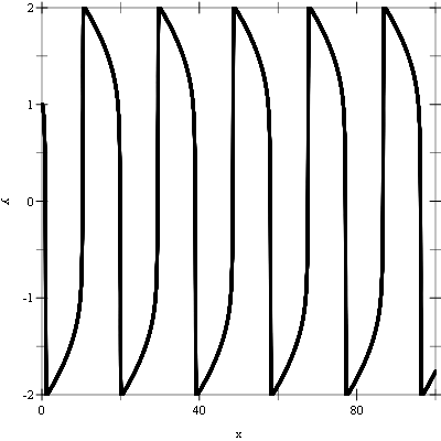
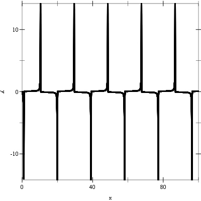
The following example integrates the above system of equations from t = 0.0 to 100.0 in increments of 0.01 using a 4th order Runge-Kutta stepping function.
The following figures show the resulting plots.


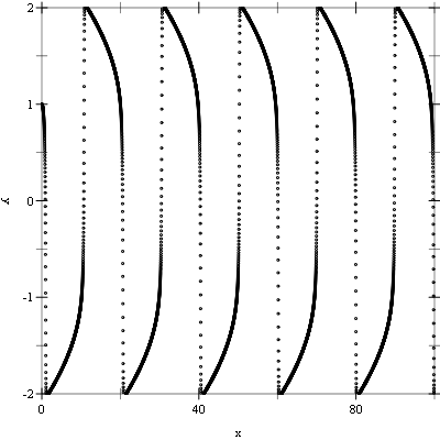
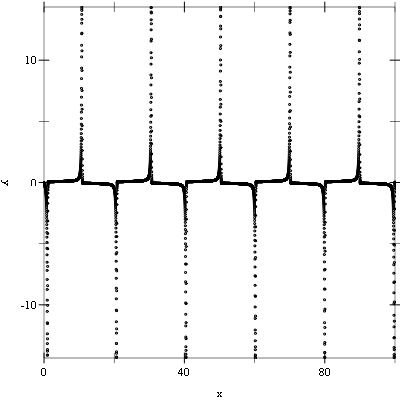
Example: The following example evolves the above system of equations from t = 0.0 to 100.0 maintaining an error in the y values of 10-6 using a 4th order Runge-Kutta stepping function.
The following shows the printed output and resulting plots.
Number of iterations = 84575 |
Number of failed steps = 352 |
