5 Special Functions

The functions described in this chapter are defined in the special-functions sub-collection of the science collection. The entire special-functions sub-collection can be made available using the form:

(require (planet williams/science/special-functions))

The individual modules in the special-functions sub-collection can also be made available as describes in the sections below.

5.1 Error Functions

The error function is described in Abramowitz and Stegun [Abramowitz64], Chapter 7. The functions are defined in the "error.ss" file in the special-functions sub-collection of the science collection and are made available using the form:

(require (planet williams/science/special-functions/error))

5.1.1 Error Function

Erf from Wolfram MathWorld.

(erf x) → (real-in -1.0 1.0)

x : real?

Computes the error function:

erf equation .

An unchecked version, unchecked-erf is also provided.

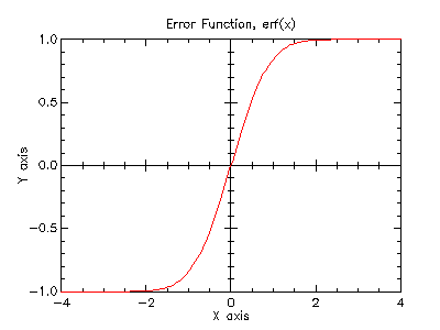
Example: Plot of (erf x) on the interval [-4, 4].

  #lang scheme
  (require (planet williams/science/special-functions/error))
  (require plot/plot)

  (plot (line erf)
        (x-min -4.0) (x-max 4.0)
        (y-min -1.0) (y-max 1.0)
        (title "Error Function, erf(x)"))

The following figure shows the resulting plot:

erf plot

5.1.2 Complementary Error Function

Erfc from Wolfram MathWorld.

(erfc x) → (real-in 0.0 2.0)

x : real?

Computes the complementary error function:

erfc equation .

An unchecked version, unchecked-erfc, is also provided.

(log-erfc x) → real?

x : real?

Computes the log of the complementary error function. An unchecked version, unchecked-log-erfc, is also provided.

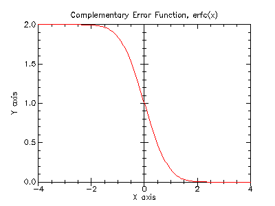
Example: Plot of (erfc x) on the interval [-4, 4].

  #lang scheme
  (require (planet williams/science/special-functions/error))
  (require plot/plot)

  (plot (line erfc)
        (x-min -4.0) (x-max 4.0)
        (y-min 0.0) (y-max 2.0)
        (title "Complementary Error Function, erfc(x)"))

The following figure shows the resulting plot:

erfc plot

5.1.3 Hazard Function

Hazard Function from Wolfram MathWorld.

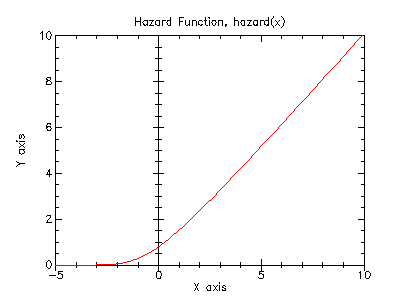
The hazard function for the normal distribution, also known as the inverse Mill’s ratio, is the ratio of the probability function, P(x), to the survival function, S(x), and is defined as:

hazard equation

(hazard x) → (>=/c 0.0)

x : real?

Computes the hazard function for the normal distribution. An unchecked version, unchecked-hazard, is also provided.

Example: Plot of (hazard x) on the interval [-5, 10].

  #lang scheme
  (require (planet williams/science/special-functions/error))
  (require plot/plot)

  (plot (line hazard)
        (x-min -5.0) (x-max 10.0)
        (y-min 0.0) (y-max 10.0)
        (title "Hazard Function, hazard(x)"))

The following figure shows the resulting plot:

hazard plot

5.2 Exponential Integral Functions

Exponential Intgral from Wolfram MathWorld.

Information on the exponential integral functions can be found in Abramowitz and Stegun [Abramowitz64], Chapter 5. The functions are defined in the "exponential-integral.ss" file in the special-functions sub-collection of the science collection are made available using the form:

(require (planet williams/science/special-functions/exponential-integral))

5.2.1 First-Order Exponential Integral

(expint-E1 x) → real?

x : real?

(expint-E1-scaled x) → real?

x : real?

Computes the exponential integral E1(x):

Unchecked versions, unchecked-expint-E1 and unchecked-expint-E1-scaled, are also provided.

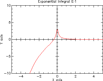
Example: Plot of (expint-E1 x) on the interval [-4, 4].

  #lang scheme
  (require (planet williams/science/special-functions/exponential-integral))
  (require plot/plot)

  (plot (line expint-E1)
        (x-min -4.0) (x-max 4.0)
        (y-min -10.0) (y-max 10.0)
        (title "Exponential Integral, E1(x)"))

The following figure shows the resulting plot:

5.2.2 Second-Order Exponential Integral

(expint-E2 x) → real?

x : real?

(expint-E2-scaled x) → real?

x : real?

Computes the second-order exponential integral E2(x):

Unchecked versions, unchecked-expint-E2 and unchecked-expint-E2-scaled, are also provided.

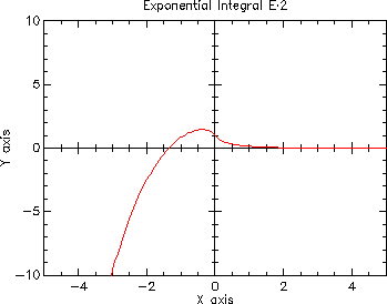
Example: Plot of (expint-E2 x) on the interval [-4, 4].

  #lang scheme
  (require (planet williams/science/special-functions/exponential-integral))
  (require plot/plot)

  (plot (line expint-E2)
        (x-min -4.0) (x-max 4.0)
        (y-min -10.0) (y-max 10.0)
        (title "Exponential Integral, E2(x)"))

The following figure shows the resulting plot:

5.2.3 General Exponential Integral

(expint-Ei x) → real?

x : real?

(expint-Ei-scaled x) → real?

x : real?

Computes the exponential integral Ei(x):

Unchecked versions, unchecked-expint-Ei and unchecked-expint-Ei-scaled, are also provided.

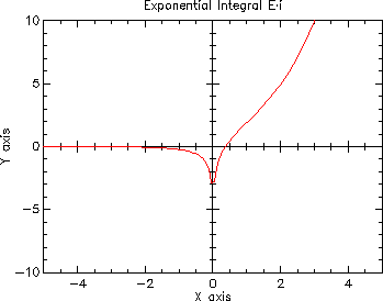
Example: Plot of (expint-Ei x) on the interval [-4, 4].

  #lang scheme
  (require (planet williams/science/special-functions/exponential-integral))
  (require plot/plot)

  (plot (line expint-Ei)
        (x-min -4.0) (x-max 4.0)
        (y-min -10.0) (y-max 10.0)
        (title "Exponential Integral, Ei(x)"))

The following figure shows the resulting plot:

5.3 Gamma and Beta Functions

The gamma functions are defined in the "gamma.ss" file in the special-functions sub-collection of the science collection and are made available using the form:

(require (planet williams/science/special-functions/gamma))

Note that the gamma functions (Section 5.3), psi functions (Section 5.4), and the zeta functions (Section 5.5) are defined in the same module, "gamma.ss". This is because their definitions are interdependent and PLT Scheme does not allow circular module dependencies.

5.3.1 Gamma Function

Gamma Function from Wolfram MathWorld.

The gamma function is defined by the integral:

It is related to the factorial function by Γ(n) = (n - 1)! for positive integer n. Further information on the gamma function can be found in Abramowitz and Stegun [Abramowitz64], Chapter 6.

(gamma x) → real?

x : real?

Computes the gamma function, Γ(x), subject to x not being a negative integer. This function is computed using the real Lanczos method. The maximum value of x such that Γ(x) is not considered an overflow is given by the constant gamma-xmax and is 171.0.

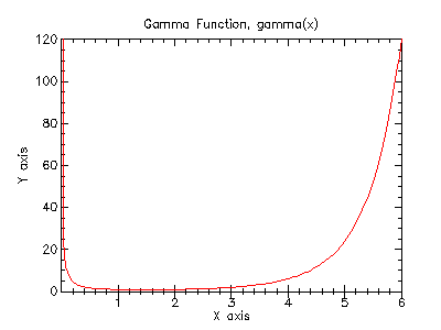
Example: Plot of (gamma x) on the interval (0, 6].

  #lang scheme
  (require (planet williams/science/special-functions/gamma))
  (require plot/plot)

  (plot (line gamma)
        (x-min 0.001) (x-max 6.0)
        (y-min 0.0) (y-max 120.0)
        (title "Gamma Function, Gamma(x)"))

The following figure shows the resulting plot:

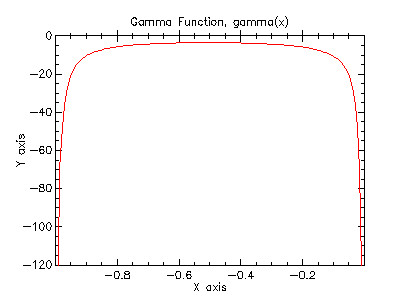
Example: Plot of (gamma x) on the interval (-1, 0).

  #lang scheme
  (require (planet williams/science/special-functions/gamma))
  (require plot/plot)

  (plot (line gamma)
        (x-min -0.999) (x-max -0.001)
        (y-min -120.0) (y-max 0.0)
        (title "Gamma Function, Gamma(x)"))

The following figure shows the resulting plot:

Log Gamma Function from Wolfram MathWorld.

(lngamma x) → real?

x : real?

Computes the logarithm of the gamma function, log Γ(x), subject to x not being a negative integer. For x < 0, the real part of log Γ(x) is returned, which is equivalent to log |Γ(x)|. The function is computed using the real Lanczos method.

(lngamma-sgn x)

→

real?

(integer-in -1 1)

x : real?

Computes the logarithm of the magnitude of the gamma function and its sign, subject to x not being a negative integer, and returns them as multiple values. The function is computed using the real Lanczos method. The value of the gamma function can be reconstructed using the relation Γ(x) = sgn × exp(resultlg), where resultlg and sgn are the returned values.

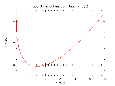
Example: Plot of (lngamma x) on the interval (0, 6].

  #lang scheme
  (require (planet williams/science/special-functions/gamma))
  (require plot/plot)

  (plot (line lngamma)
        (x-min 0.001) (x-max 6.0)
        (y-min 0.0) (y-max 5.0)
        (title "Log Gamma Function, log Gamma(x)"))

The following figure shows the resulting plot:

(gamma-inv x) → real?

x : real?

Computes the reciprocal of the gamma function, 1/Γ(x), using the real Lanczos method.

5.3.2 Regulated Gamma Function

The regulated gamma function is given by

(gammastar x) → real?

x : (>/c 0.0)

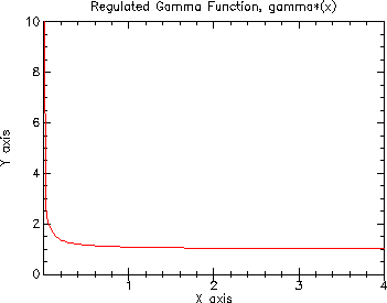
Computes the regulated gamma function, Γ*(x), for x > 0.

Example: Plot of (gammastar x) on the interval (0, 4].

  #lang scheme
  (require (planet williams/science/special-functions/gamma))
  (require plot/plot)

  (plot (line gammastar)
        (x-min 0.001) (x-max 4.0)
        (y-min 0.0) (y-max 10.0)
        (title "Regulated Gamma Function, Gamma*(x)"))

The following figure shows the resulting plot:

5.3.3 Incomplete Gamma Function

Incomplete Gamma Function from Wolfram MathWorld.

(gamma-inc-Q a x) → real?

a : (>/c 0.0)

x : (>=/c 0.0)

Computes the normalized incomplete gamma function,

for a > 0 and x ≥ 0.

(gamma-inc-P a x) → real?

a : (>/c 0.0)

x : (>=/c 0.0)

Computes the complementary normalized incomplete gamma function,

for a > 0 and x ≥ 0.

(gamma-inc a x) → real?

a : real?

x : (>=/c 0.0)

Computes the unnormalized incomplete gamma function,

for a real and x ≥ 0.

5.3.4 Factorial Function

The factorial of a positive integer n, n!, is defined as n! = n × (n - 1) × ... × 2 × 1. By definition, 0! = 1. The related function is related to the gamma function by Γ(n) = (n - 1)!.

(fact n) → (>=/c 1.0)

n : natural-number/c

Computes the factorial of n, n!.

(lnfact n) → (>=/c 0.0)

n : natural-number/c

Computes the logarithm of the factorial of n, log n!. The algorithm is faster than computing ln Γ(n + 1) via lngamma for n < 170, but defers for larger n.

5.3.5 Double Factorial Function

The double factorial of n, n!!, is defined as n! = n × (n - 2) × (n - 4) × .... By definition, -1!! = 0!! = 1.

(double-fact n) → (>=/c 1.0)

n : natural-number/c

Computes the double factorial of n, n!!.

(lndouble-fact n) → (>=/c 0.0)

n : natural-number/c

Computes the logarithm of the double factorial of n, log n!!.

5.3.6 Binomial Coefficient Function

The binomial coefficient, n choose m, is defined as:

(choose n m) → (>=/c 1.0)

n : natural-number/c

m : natural-number/c

Computes the binomial coefficient for n and m, n choose m.

(lnchoose n m) → (>=/c 0.0)

n : natural-number/c

m : natural-number/c

Computes the logarithm of the binomial coefficient for n and m, log (n choose m).

5.3.7 Beta Functions

Beta Function from Wolfram MathWorld.

(beta a b) → real?

a : (>/c 0.0)

b : (>/c 0.0)

Computes the beta function,

for a > 0 and b > 0.

(lnbeta a b) → real?

a : (>/c 0.0)

b : (>/c 0.0)

Computes the logarithm of the beta function, log Β(a, b), for a > 0 and b > 0.

5.4 Psi Functions

The psi functions are defined in the "gamma.ss" file in the special-functions sub-collection of the science collection and are made available using the form:

(require (planet williams/science/special-functions/gamma))

5.4.1 Psi (Digamma) Functions

Digamma Function from Wolfram MathWorld.

(psi-int n) → real?

n : (integer-in 1 +inf.0)

Computes the digamma function, Ψ(n), for positive integer n. The digamma function is also called the Psi function.

(psi x) → real?

x : real?

Returns the digamma function, Ψ(x), for general x, x ≠ 0.

(psi-1piy y) → real?

y : real?

Computes the real part of the digamma function on the line 1 + iy, Re Ψ(1 + iy).

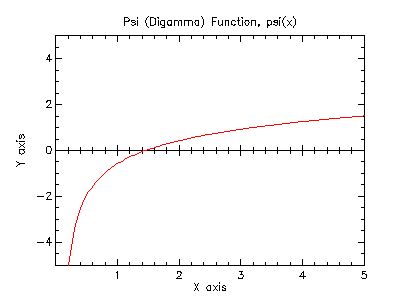
Example: Plot of (psi x) on the interval (0, 5].

  #lang scheme
  (require (planet williams/science/special-functions/gamma))
  (require plot/plot)

  (plot (line psi)
        (x-min 0.001) (x-max 5.0)
        (y-min -5.0) (y-max 5.0)
        (title "Psi (Digamma) Function, Psi(x)"))

The following figure shows the resulting plot:

5.4.2 Psi-1 (Trigamma) Functions

Trigamma Function from Wolfram MathWorld.

(psi-1-int n) → real?

n : (integer-in 1 +inf.0)

Computes the trigamma function, Ψ′(n), for positive integer n.

(psi-1 x) → real?

x : real?

Computes the trigamma function, Ψ′(x), for general x.

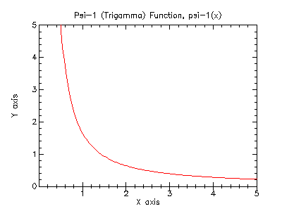
Example: Plot of (psi-1 x) on the interval (0, 5].

  #lang scheme
  (require (planet williams/science/special-functions/gamma))
  (require plot/plot)

  (plot (line psi-1)
        (x-min 0.001) (x-max 5.0)
        (y-min 0.0) (y-max 5.0)
        (title "Psi-1 (Trigamma) Function, Psi-1(x)"))

The following figure shows the resulting plot:

5.4.3 Psi-n (Polygamma) Functions

Polygamma Function from Wolfram MathWorld.

(psi-n n x) → real?

n : natural-number/c

x : (>/c 0.0)

Computes the polygamma function, Ψm(x), for m ≥ 0, x > 0.

Example: Plot of (psi-n n x) for n = 3 on the interval (0, 5].

  #lang scheme
  (require (planet williams/science/special-functions/gamma))
  (require plot/plot)

  (plot (line (lambda (x) (psi-n 3 x)))
        (x-min 0.001) (x-max 5.0)
        (y-min 0.0) (y-max 10.0)
        (title "Psi-n (Polygamma) Function, Psi-n(3, x)"))

The following figure shows the resulting plot:

5.5 Zeta Functions

The Riemann zeta function is defined in Abramowitz and Stegun [Abramowitz64], Section 23.3. The zeta functions are defined in the "gamma.ss" file in the special-functions subcollection of the science collection are are made available using the form:

(require (planet williams/science/special-functions/gamma))

5.5.1 Riemann Zeta Functions

Riemann Zeta Function from Wolfram MathWorld.

The Riemann zeta function is defined by the infinite sum:

(zeta-int n) → real?

n : integer?

Computes the Reimann zeta function, ζ(n), for integer n, n ≠ 1.

(zeta s) → real?

s : real?

Computes the Riemann zeta function, ζ(s), for arbitrary s, s ≠ 1.

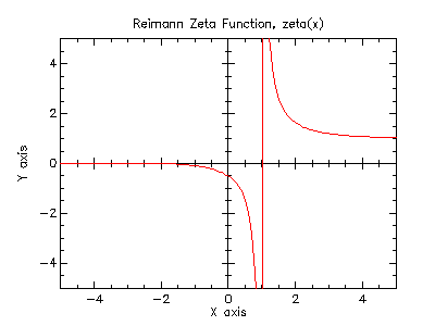
Example: Plot of (zeta x) on the interval [-5, 5].

  #lang scheme
  (require (planet williams/science/special-functions/gamma))
  (require plot/plot)

  (plot (line zeta)
        (x-min -5.0) (x-max 5.0)
        (y-min -5.0) (y-max 5.0)
        (title "Riemann Zeta Function, zeta(x)"))

The following figure shows the resulting plot:

5.5.2 Riemann Zeta Functions Minus One

For large positive arguments, the Riemann zeta function approached one. In this region the fractional part is interesting and, therefore, we need a function to evaluate it explicitly.

(zetam1-int n) → real?

n : integer?

Computes ζ(n) - 1 for integer n, n ≠ 1.

(zetam1 s) → real?

s : real?

Computes ζ(s) - 1 for argitrary s, s ≠ 1.

5.5.3 Hutwitz Zeta Function

Hurwitz Zeta Function from Wolfram MathWorld.

The Hurwitz zeta function is defined by:

(hzeta s q) → real?

s : (>/c 1.0)

q : (>/c 0.0)

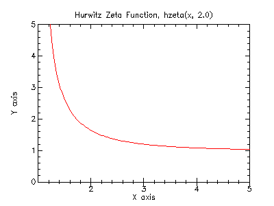
Computes the Hurwitz zeta function, ζ(s, q), for s > 1, q > 0.

Example: Plot of (hzeta x 2.0) on the interval (1, 5].

  #lang scheme
  (require (planet williams/science/special-functions/gamma))
  (require plot/plot)

  (plot (line (lambda (x) (hzeta x 2.0)))
        (x-min 1.001) (x-max 5.0)
        (y-min 0.0) (y-max 5.0)
        (title "Hutwitz Zeta Function, hzeta(x, 2.0)"))

The following figure shows the resulting plot:

5.5.4 Eta Functions

Dirichlet Eta Function from Wolfram MathWorld.

The eta function is defined by:

(eta-int n) → real?

n : integer?

Computes the eta function, η(n), for integer n.

(eta s) → real?

s : real?

Computes the eta function, η(s), for arbitrary s.

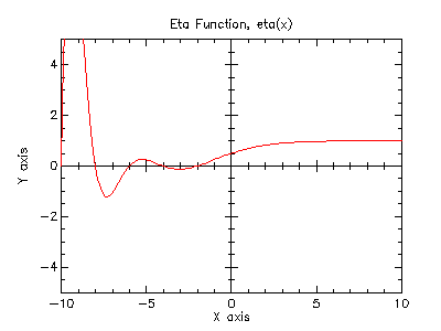
Example: Plot of (eta x) on the interval [-10, 10].

  #lang scheme
  (require (planet williams/science/special-functions/gamma))
  (require plot/plot)

  (plot (line eta)
        (x-min -10.0) (x-max 10.0)
        (y-min -5.0) (y-max 5.0)
        (title "Eta Function, eta(x)"))

The following figure shows the resulting plot:

← prev up next →

1	Introduction
2	Using the Science Collection
3	Error Handling
4	Mathematical Functions
5	Special Functions
6	Random Number Generation
7	Random Number Distributions
8	Statistics
9	Histograms
10	Ordinary Differential Equations
11	Chebyshev Approximations
12	GNU Free Documentation License
	Bibliography
	Index

5.1	Error Functions
5.2	Exponential Integral Functions
5.3	Gamma and Beta Functions
5.4	Psi Functions
5.5	Zeta Functions